Walkthrough#
The MEA GUI allows you to detect and quantify Seizure-Like Events (SLEs) and other neural activity patterns from your processed Multi-Electrode Array (MEA) recordings. This page walks you through the full workflow— from opening files to running analyses and viewing results.
Whether you’re an experienced neuroscience researcher or an undergraduate research assistant, this step-by-step guide will help you understand and use the analysis tools effectively.
1. Open File#
Before analyzing data, load your MEA recording into the GUI.
Steps to Open a File:#
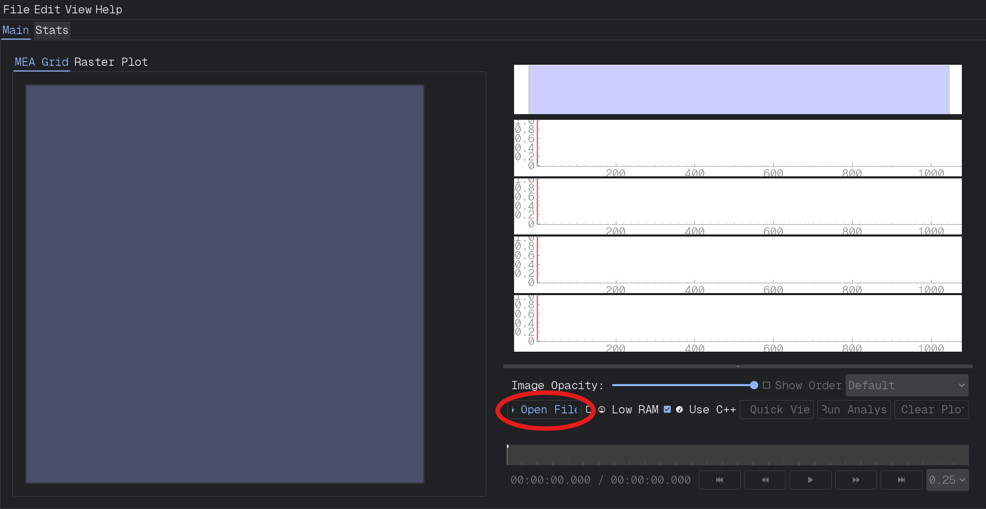
Select the
Open Filebutton just below the graphs on the right-hand side of the screen.
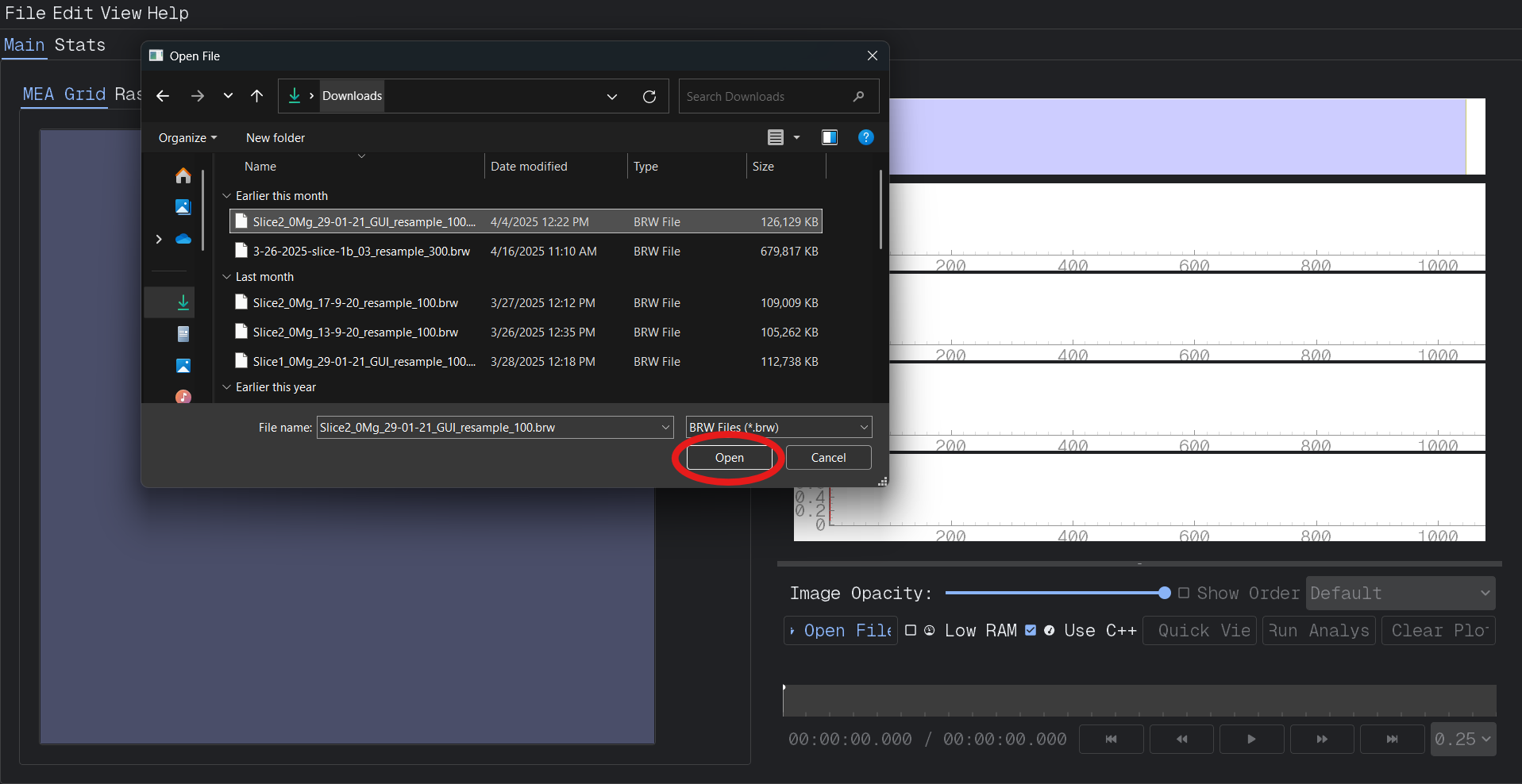
Browse to the
.brwMEA file you want to open and clickOpen.
Select the
Quick Viewbutton to the right of theOpen Filebutton.
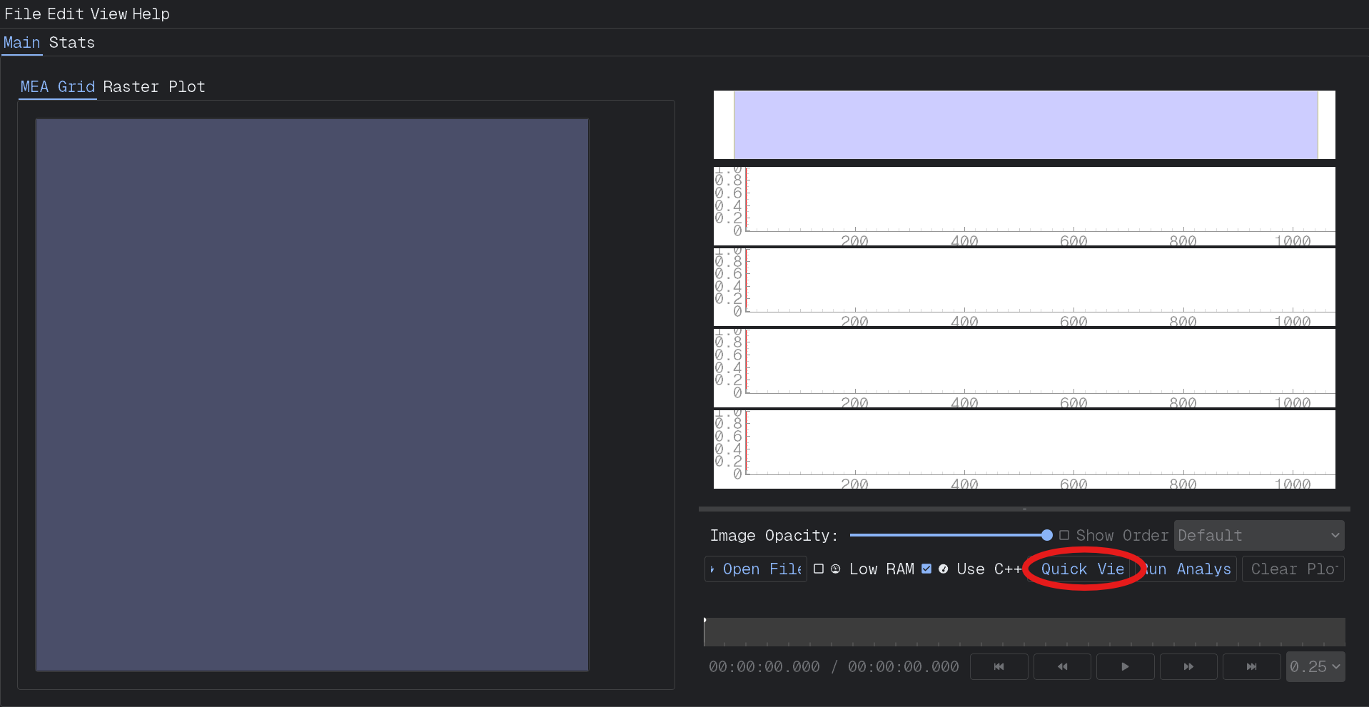
Once opened, a preview of the data will appear in the left-hand MEA Grid pane.
Note
Files should be pre-processed using the GUI’s processing tools or imported from compatible sources. Raw files without timestamps or signal alignment may not load properly.
2. Quick View#
After opening your MEA file, you should visually check your data to ensure quality before running any analysis.
Tip
It’s a good practice to scan through the recording for any major noise or missing data before starting an analysis.
Note
Quick View vs. Run Analysis
Use Quick View if you want to watch live LFP traces for each channel or visualize activity in real time on the false color map. This is ideal for quickly inspecting the recording without doing detailed analysis.
Use Run Analysis if you want to detect seizures, track discharges, and generate quantitative results. This runs the full analysis pipeline, and from here you can save your results from further review.
First, choose what you want to view…#
Location Field Potential (LFP) Traces: Click any electrode on the MEA Grid to view its Local Field Potential (LFP) trace over time. The LFP trace plot reflects slow voltage fluctuations from groups of neurons near the selected electrode, and it is helpful for spotting large discharges or seizure onset patterns.
As a discharge propagates across the slice, the false color map on the MEA Grid dynamically updates to show which electrodes are active and when. Each square’s color reflects the relative signal intensity at that electrode:
Brighter or warmer colors (e.g., red, yellow) represent stronger or more recent activity.
Cooler colors (e.g., blue) represent lower or older activity.
The map refreshes continuously to show real-time propagation across the brain slice.
This visualization lets you track how a discharge spreads — from initiation, through propagation, to termination — as it recruits different regions.
Once you’ve observed a discharge progressing across the array:
Watch the false color map closely to identify where the discharge begins and how it travels.
Click the electrode at the earliest point of activity — where the discharge likely originates.
Press the number key 1 to save that LFP trace into Trace Box 1. (Denoted by a red shape in both the selected channel and its associated trace box.)
Then, follow the discharge’s path by selecting subsequent electrodes along its propagation route. - Press 2 and 3 to save intermediate points.
Finally, identify where the discharge appears to stop or weaken, and save that electrode’s trace to Trace Box 4.
This process lets you reconstruct how the event evolved spatially across the slice.
Tip
By saving LFP traces from electrodes at key points along the path of the discharge, you can compare the waveform shape and timing across locations — helpful for understanding network recruitment and seizure spread.
Note
To learn more about navigating trace plots, saving multiple channels, and using the analysis views in more depth, see the Right Pane documentation.
Raster Plots: Select the Raster Plot tab to display spike trains across electrodes. (Use this to check for active electrodes and obvious artifacts.)
Add something here about:
Edit Raster Settings, modify theSpike Thresholdbased on what the recording looks like in the raster plot.
Explore Raster Plots 📈
Curious about how spikes are visualized across electrodes? See the section on Raster Plots for a deeper dive into interpreting activity on the MEA grid.
3. Run Analysis#
Press the Run Analysis button at the bottom of the Analysis tab.
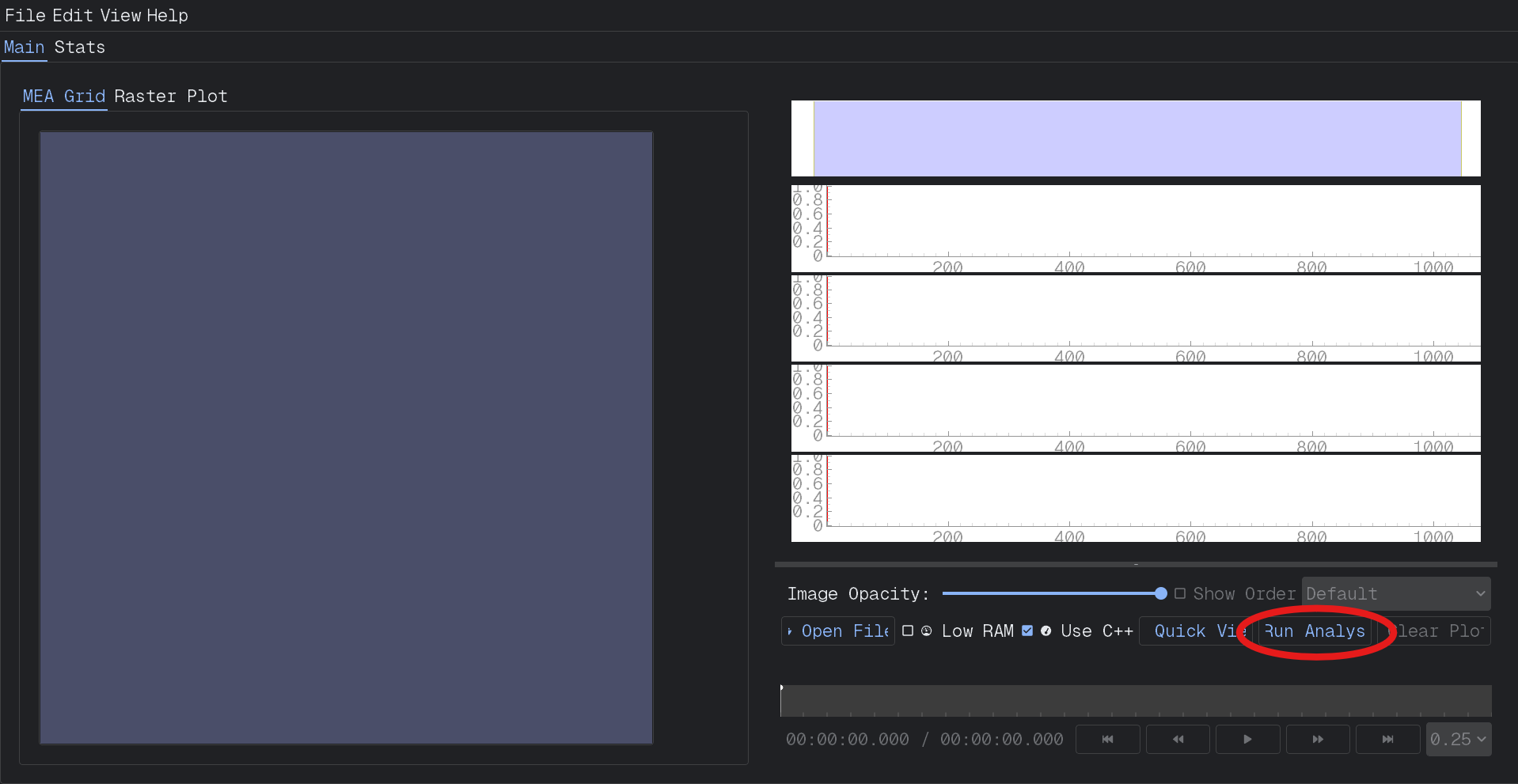
What Happens:
It scans for Seizure-Like Events (SLEs).
Analysis usually takes 2-5 minutes per file, depending on the available RAM, file size, and downsample ratio.
Tip
Monitor progress in the status bar. You can cancel ongoing analysis with the Stop button if needed.
4. Configure Analysis Settings#
Note
Add material here after adjusting layout of analysis settings.
5. View Results#
Once complete, you’ll see:
SLE timeline: Start and end times of detected seizure-like events.
Event list: Each event’s duration, Amplitude, and electrode involvement.
Raster plots: With detected events highlighted.
Results are automatically saved and can be exported for further processing.
Tip
🧭 Want to explore how a discharge spreads across the slice?
After completing analysis, you can dive deeper using the Discharge Propagation Tracking tool to visualize spatial dynamics of seizure-like events.
Common Issues#
File won’t open? Confirm it is processed and in
.brwor.h5format.Analysis returns no events? Try lowering your Threshold detection value.
Too many false events? Consider raising your Threshold detection value or increasing the analysis Window size.